Use case Guide - Scenario 5 - Live dashboards#
This document is meant to guide the user through Scenario 5 - Automated dashboards. As disussed in the use case description, the goal is to provide an automated weather forecast dashboard which fetches data from an open API on a daily basis (for the city of Brussels). The guide will be a step by step tutorial towards such objective. More in detail, each subsection covers a step of the approach, namely:
- Step 1: Initialize the resources.
- Step 2: Retrieve the PostgreSQL host address.
- Step 3: Set up the data pipeline - Data fetching & DAG script.
- Step 4: Initiate the data pipeline - Airflow.
- Step 5: Create the dashboard.
Use case files#
| Code |
|---|
| Use-case code - Scenario 5 - Live dashboards |
| Use-case dag - Scenario 5 - Live dashboards |
Step 1: Initialize the resources#
As first step, the user should inizialize the required resources. More in particular, four instances should be launched: - Apache Airflow - Jupyterlab - PostgreSQL - Apache Superset
Initialize the Jupyterlab/Airflow instance#
- Go on the Service Catalog section of the Portal.
- Click on the button Launch on the Jupyterlab/Airflow badge.
- Assign a name to the instance and select a group from the ones available in the list.
- Select the Default configuration.
- Copy the auto-generated password. This will be needed to access the instance in the later stage. (NB: Instance credentials are automatically saved and acessible on the My Data section of the portal).
- Select the NFS PVC name corresponding to the DSL group selected at point 3.
- Launch the instance by clicking on the launch button.
Initialize the Postgres SQL instance#
- Go on the Service Catalog section of the Portal.
- Click on the button Launch on the PostgreSQL badge.
- Assign a name to the instance and select a group from the ones available in the list.
- Select the micro configuration.
-
Copy the auto-generated Admin password. From now on, the PostgreSQL password will be referenced as:
<postgreSQLPassword> -
Launch the instance by clicking on the launch button.
Initialize the Apache Superset instance#
- Go on the Service Catalog section of the Portal.
- Click on the button Launch on the Apache Superset badge.
- Assign a name to the instance and select a group from the ones available in the list.
- Select the micro configuration.
- Set your Admin username, Admin email, Admin firstname and Admin lastname.
- Copy the auto-generated password. This will be needed to access the instance in the later stage. (NB: Instance credentials are automatically saved and acessible on the My Data section of the portal).
- Launch the instance by clicking on the launch button.
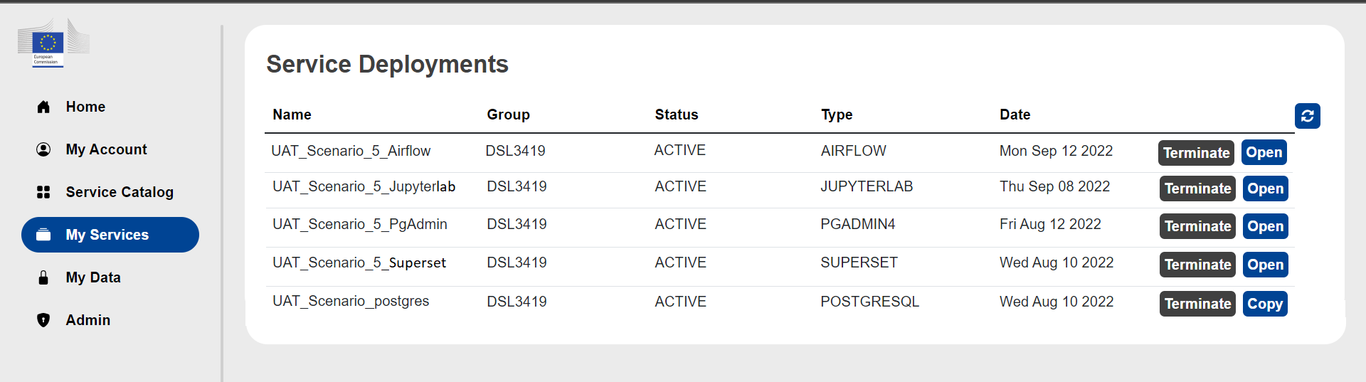
After having launch the instances, go on the My Services section of the portal to verify that all the deployed services are up and running (all three instances should be in status ACTIVE).
Step 2: Retrieve the PostgreSQL host address#
- From the My Services section of the portal, click on the Copy button of the PostgreSQL instance to copy the host address of the instance in the clipboard.
- The PostgreSQL host address is in the format:
<postgresSQLHost>:5432
Step 3: Set up the data pipeline - Data fetching & DAG script#
-
Download the data fetching script and the DAG script:
- Data fetching script: UAT_Scenario_5.py
- DAG script: UAT_Scenario_5_DAG.py
Please note that both scripts are commented for a better understanding of each step performed.
-
Open the Data fetching script with a text editor and edit the code at point 3) Define the DB engine parameters in the following way:
- Substitute
<postgreSQLPassword>with the PostgreSQL password (see Initialize the Postgres SQL instance - point 5.); - Substitute
<postgresSQLHost>with the PostgreSQL host address (see Step 2: Retrieve the PostgreSQL host address - point 2. )
Please note that each line that needs to be edited is commented with "# EDIT THIS LINE" 3. From the My Services section of the portal, click on the Open button to access the Jupyterlab instance. 4. Login into your Jupyterlab instance with the access credentials defined in the configuration. 5. Upload into the dags folder the just edited Data fetching script and the DAG script.
- Substitute
DISCLAIMER: Please note that is important NOT to run the two scripts on Jupyterlab but just to upload them. As a matter of fact, running the DAG script on Jupyterlab would cause the override of the configuration that allows to connect Airflow to Jupyterlab.
Step 4: Initiate the data pipeline - Airflow#
- From the My Services section of the portal, click on the Open button to access the Airflow instance.
- Login into your Airflow instance with the access credentials defined in the configuration.
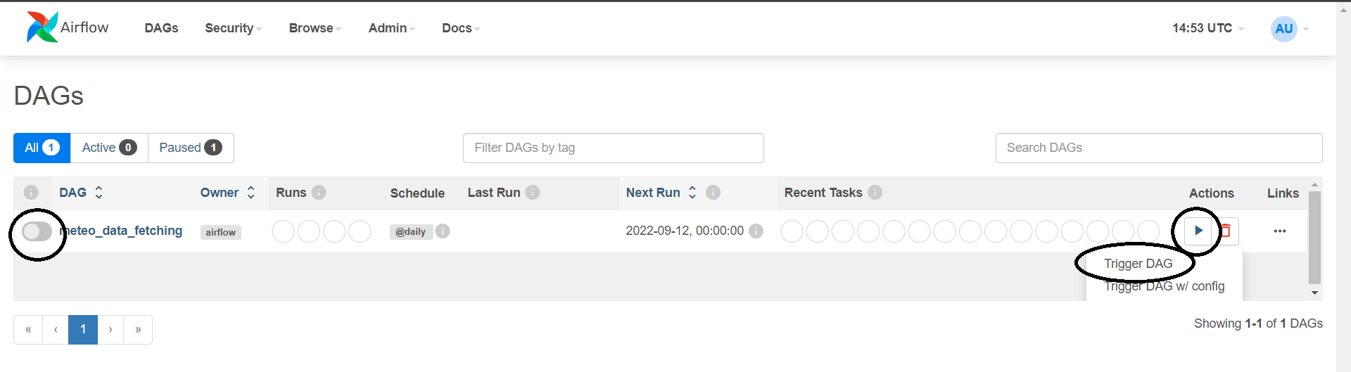
- In the DAG section of Airflow, you should see the meteo_data_fetching DAG. Please note that, accordingly to the configuration made on the DAG Script, this DAG is scheduled daily execute (Schedule) the Data fetching script.
- Click on the toggle on the top-left to activate the DAG (see image here below).
- Click on the play button and then on Trigger DAG to manually trigger its execution (see image here below).
- Wait a few seconds and you should see the indication that the DAG has been executed succesfully:
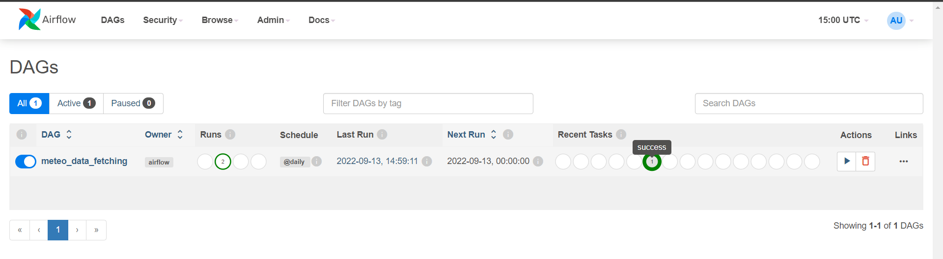
- The succesful execution of this DAG imply that 2 new tables (hourly data, metadata) have been created and filled in on our PostgreSQL DB.
Step 5: Create the dashboard#
Add the DB and datasets#
- From the My Services section of the portal, click on the Open button to access the Superset instance.
- Login into your Superset instance with the access credentials defined in the configuration.
- In the navbar, click on Data > Databases.
- Click on the " + DATABASE " button. This will open the Connect a database tool that will allow us to connect the Postgres SQL database to Apache Superset.
- Select PostgreSQL as database to connect.
- Enter the required PostgreSQL credentials:
- HOST: input the
<postgresSQLHost> - PORT: 5432
- DATABASE NAME: postgres
- USERNAME: postgres
- PASSWORD: input the
<postgreSQLPassword>
- HOST: input the
- Click on Connect.
- In the navbar, click on Data > Datasets.
- Click on the " + DATASETS " button. This will open the Add dataset tool that will allow us to add the tables from the newly connected Postgres SQL database.
- In the DATABASE field, select the database that has been connected to Apache Superset in the previous step.
- In the SCHEMA field, select public.
- In the SEE TABLE SCHEMA field, select the table hourly_data.
- Repeat the same operation to add the metadata dataset.
- For the hourly_data dataset, in the Actions section press on the Edit icon.
- Go on COLUMNS and tick the property Is temporal and Default datetime for the column hourly_time. This will allow Apache Superset to deal with such column as a temporal dimension, and this will be needed for all time-related data visualizations (eg. bar charts, time series, ...).
Create the charts#
- To create a new chart, click on Charts on the Superset navbar, then click on the + CHART button.
- Choose the hourly_data dataset.
A list of charts is here below proposed:
1. Weekly temperature forecast#
- Select the Time-series Line Chart and click on Create New Chart.
- By default, the TIME COLUMN should be hourly_time with Original Value as TIME GRAIN.
- In the QUERY section of the DATA tab, create a new metric as follows:
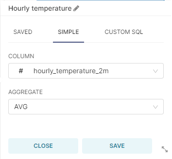
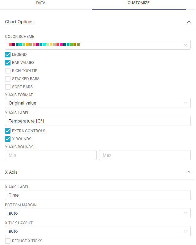
- In the CUSTOMIZE tab, have the following settings:
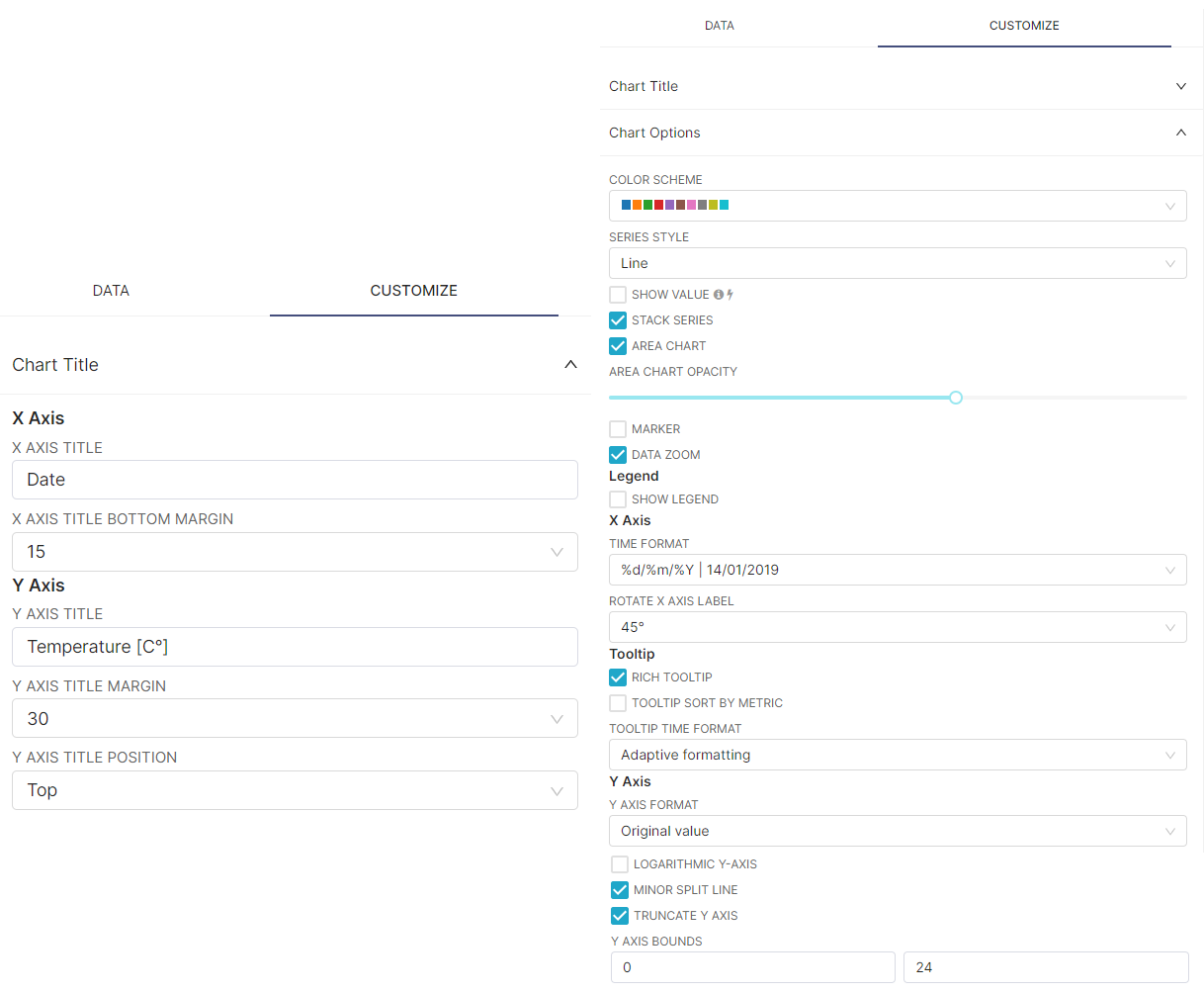
- Click on the SAVE button, assign a CHART NAME and click on SAVE.
2. Temperature vs. Perceived Temperature#
- Select the Bar Chart and click on Create New Chart.
- By default, the TIME COLUMN should be hourly_time.
- In the QUERY section of the DATA tab, create two new metrics as follows:
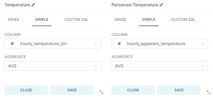
And select hourly_time as SERIES.
- In the CUSTOMIZE tab, have the following settings:
- Click on the SAVE button, assign a CHART NAME and click on SAVE.
3. Weekly Average Temperature with trendline and Weekly Min/Max temperature, cloud coverage, pressure level, rain volume#
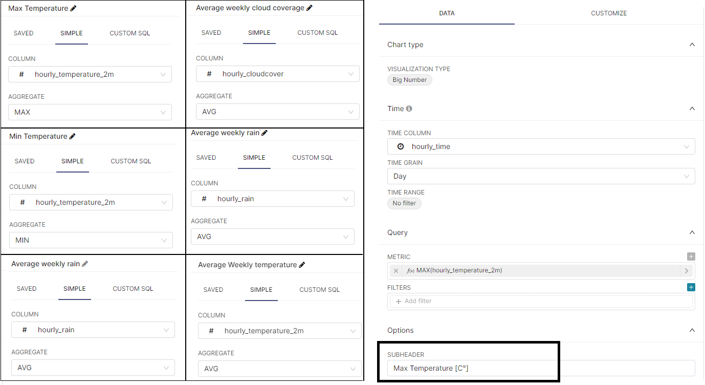
- Select the Big Number and click on Create New Chart (for the Weekly Average Temperature with trendline, select Big Number with Trendline instead).
- By default, the TIME COLUMN should be hourly_time with Day as TIME GRAIN.
- Create four different charts with the following defined metrics. Please note that you can add a sub-header as caption of the big number showed in the chart:
- Click on the SAVE button, assign a CHART NAME and click on SAVE.
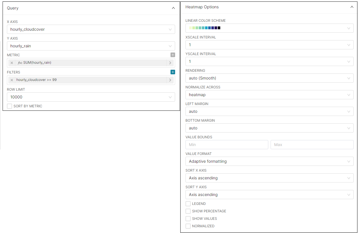
4. Heatmap - Cloud coverage vs. Rain volume#
- Select the Heatmap and click on Create New Chart .
- By default, the TIME COLUMN should be hourly_time.
- In the DATA tab, have the following settings:
- Click on the SAVE button, assign a CHART NAME and click on SAVE.
Create the dashboard and populate it with the charts#
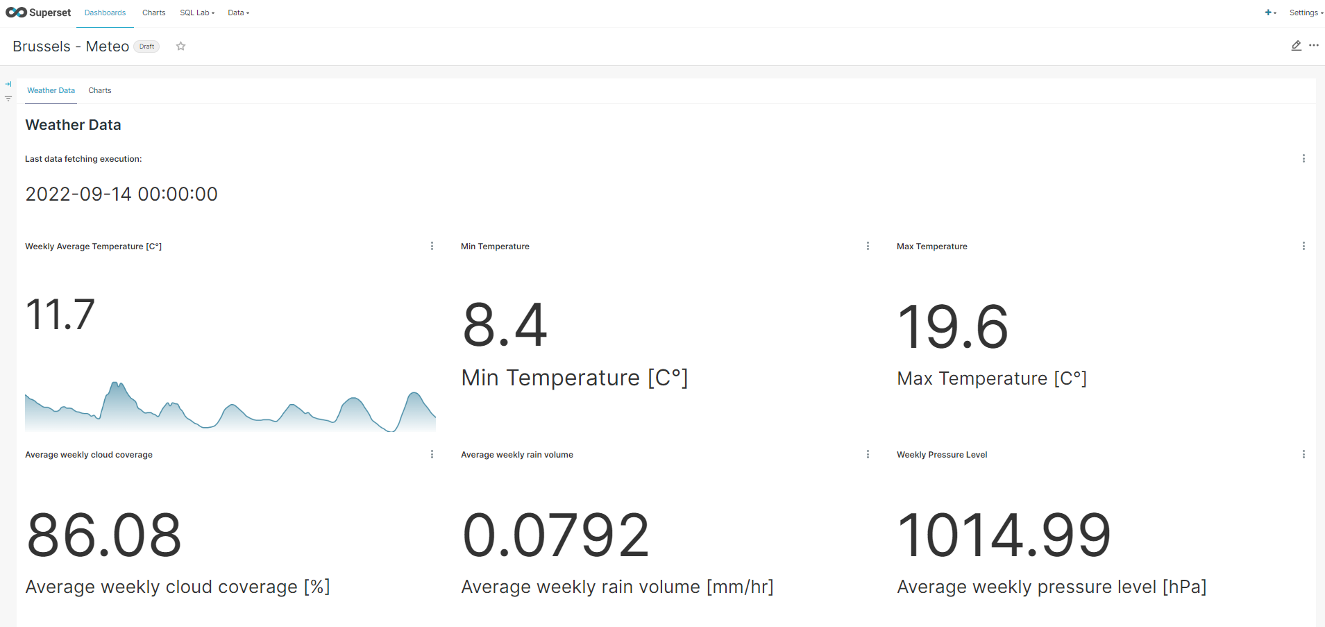
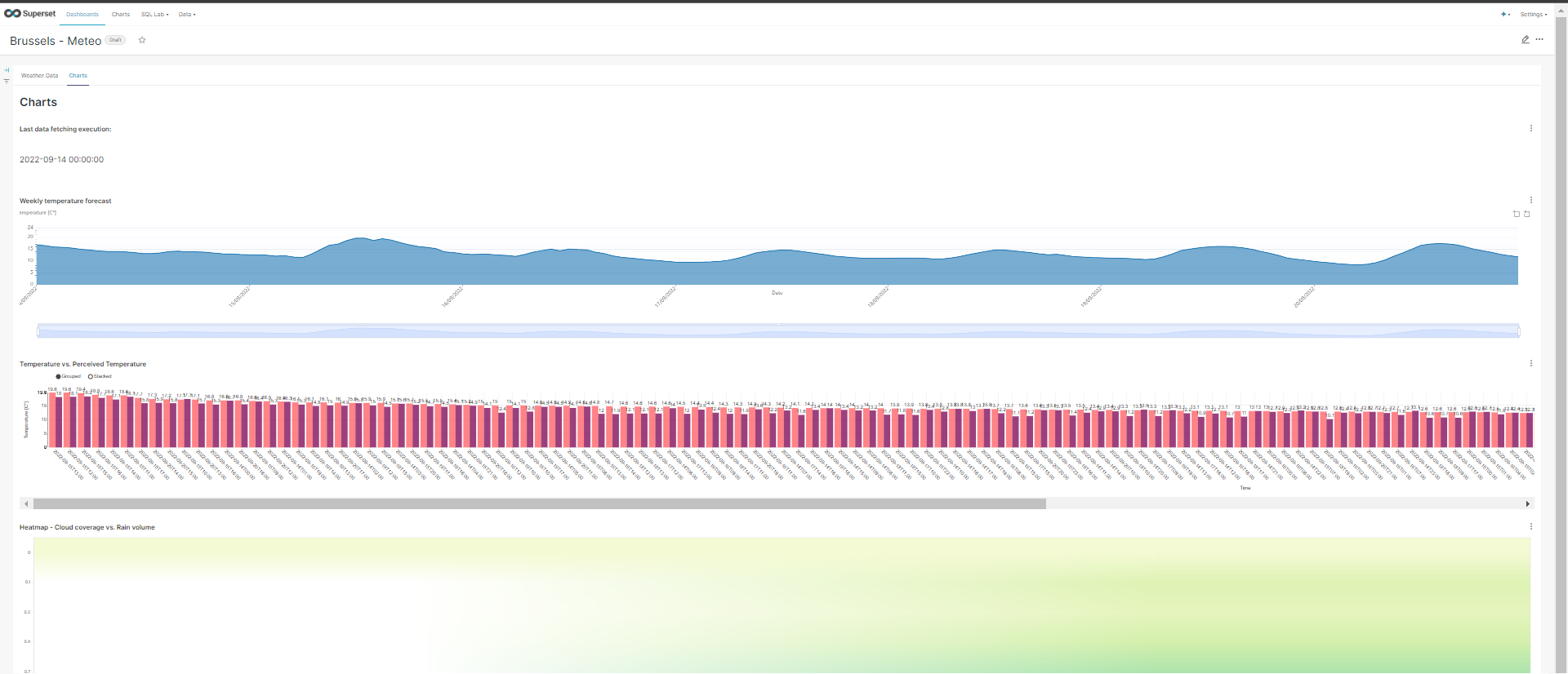
- Click on Dashboards on the navbar and click on the "+ DASHBOARD" button to add a new dashboard. Assign the dashboard a title (i.e. Brussels - Meteo)
- From the Components section, drag and drop the Tabs element. Then, create two new tabs: one will contain the big number charts and the other the plot charts. Assign names to the tabs (i.e. Weather Data and Charts).
- In the first tab, add all Big Number charts by dragging-dropping them from the Charts section.
- In the second tab, add all plot charts by dragging-dropping them from the Charts section.
- Here a dashboard created as example for the final result: